Overview
The year 2017 was a period of scientific breakthroughs in deep learning, with the publication of numerous research papers. Every year seems like a big leap toward artificial general intelligence, or AGI.
One exciting development involves generative modelling and the use of Wasserstein GANs (Generative Adversarial Networks). An influential paper on the topic has completely changed the approach to generative modelling, moving beyond the time when Ian Goodfellow published the original GAN paper.
Why Wasserstein GANs are such a big deal:
- With Wasserstein GAN, you can train the discriminator to convergence. If true, it would totally remove the need to balance generator updates with discriminator updates, as earlier the updates of generator and discriminator were happening with no correlation to each other.
- The initial paper (Soumith et al.) proposed a new GAN training algorithm that works well on the commonly used GAN datasets.
- Usually theory justified papers don’t provide good empirical results, but the training algorithm mentioned in the paper is backed up by theory and it explains why WGANs work so much better.
Introduction
This paper differs from earlier work: the training algorithm is backed up by theory, and few examples exist where theory-justified papers gave good empirical results. The big thing about WGANs is that developers can train their discriminator to convergence, which was not possible earlier. Doing this eliminates the need to balance generator updates with discriminator updates.
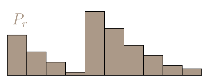
What is Earth Mover’s Distance?
When dealing with discrete probability distributions, the Wasserstein Distance is also known as Earth mover’s distance (EMD). Imagining different heaps of earth in varying quantities, EMD would be the minimal total amount of work it takes to transform one heap into another. Here, work is defined as the product of the amount of earth being moved and the distance it covers. Two discrete probability distributions are usually defined as Pr and P(theta).
Pr comes from unknown distribution, and the goal is to learn P(theta) that approximates Pr.
Calculation of EMD is an optimization process with infinite solution approaches; the challenge is to find the optimal one.
One approach would be to directly learn probability density function P(theta). This would mean that P(theta) is some differentiable function that can be optimized by maximum likelihood estimation. To do that, minimize the KL (Kullback–Leibler) divergence KL(Pr||(P(theta)) and add a random noise to P(theta) when training the model for maximum likelihood estimation. This ensures that distribution is defined elsewhere; otherwise, if a single point lies outside P(theta), the KL divergence can explode.
Adversarial training makes it hard to see whether models are training. It has been shown that GANs are related to actor-critic methods in reinforcement learning. Learn More.
Kullback–Leibler and Jensen–Shannon Divergence
- KL (Kullback–Leibler) divergence measures how one probability distribution P diverges from a second expected probability distribution Q.
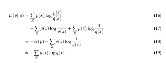
- We drop −H(p) going from (18) − (19) because it is a constant. We can see if we minimize the LHS (Left-hand side), we are maximizing the expectation of log q(x) over the distribution p. Therefore, minimizing the LHS is maximizing the RHS, which is maximizing the log-likelihood of the data.
DKL achieves the minimum zero when p(x) == q(x) everywhere.
It is noticeable from the formula that KL divergence is asymmetric. In cases where P(x) is close to zero, but Q(x) is significantly non-zero, the q’s effect is disregarded. It could cause buggy results when the intention was just to measure the similarity between two equally important distributions.
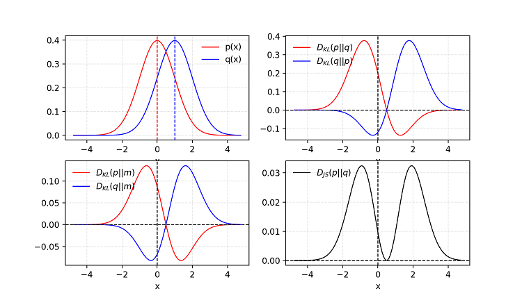
- Jensen–Shannon Divergence is another measure of similarity between two probability distributions. JS (Jensen–Shannon) divergence is symmetric and relatively smoother and is bounded by [0,1].
Given two Gaussian distributions, P with mean=0 and std=1 and Q with mean=1 and std=1. The average of two distributions is labelled as m=(p+q)/2. KL divergence DKL is asymmetric but JS divergence DJS is symmetric.
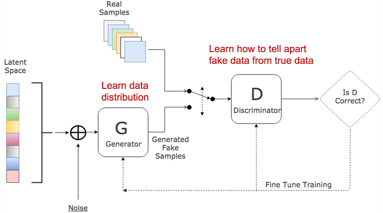
Generative Adversarial Network (GAN)
GAN consists of two models:
- A discriminator D estimates the probability of a given sample coming from the real dataset. It works as a critic and is optimized to tell the fake samples from the real ones.
- A generator G outputs synthetic samples given a noise variable input z (z brings in potential output diversity). It is trained to capture the real data distribution so that its generative samples can be as real as possible, or in other words, it can trick the discriminator to offer a high probability.
Use Wasserstein Distance as GAN Loss Function
It is almost impossible to exhaust all the joint distributions in Π(pr,pg) to compute infγ∼Π(pr,pg). Instead, the authors proposed a smart transformation of the formula based on the Kantorovich-Rubinstein duality:
One big problem involves maintaining the K-Lipschitz continuity of fw during the training to make everything work out. The paper presented a simple but very practical noteworthy trick: after the gradient gets updated, clamping the weights w to a small window is required, such as [−0.01,0.01], resulting in a compact parameter space W; and thus, fw obtains it’s lower and upper bounds in order to preserve the Lipschitz continuity.
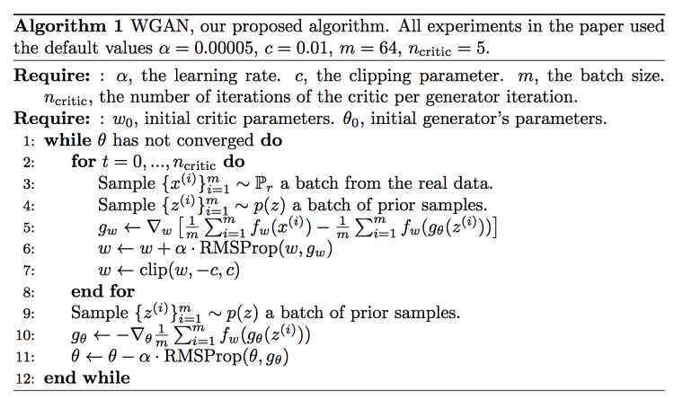
Compared to the original GAN algorithm, the WGAN undertakes the following changes:
- After every gradient update on the critic function, we are required to clamp the weights to a small fixed range is required, usually [−c,c].
- Use a new loss function derived from the Wasserstein distance. The discriminator model does not play as a direct critic but rather a helper for estimating the Wasserstein metric between real and generated data distributions.
Empirically the authors recommended usage of RMSProp optimizer on the critic, rather than a momentum-based optimizer such as Adam which could cause instability in the model training.
Improved GAN Training
The following suggestions are proposed to help stabilize and improve the training of GANs.
- Adding noises — Based on the discussion in the previous section, it is now known that Pr and Pg are disjointed in a high dimensional space and they may become the reason for the problem of vanishing gradient.To synthetically “spread out” the distribution and to create higher chances for two probability distributions to have overlaps, one solution is to add continuous noises onto the inputs of the discriminator D.
- One-sided label smoothing — When we are feeding the discriminator, instead of providing the labels as 1 and 0, this paper proposed using values such as 0.9 and 0.1. This will help in reduce the vulnerabilities in Network.
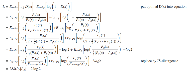
Wasserstein metric is proposed to replace JS divergence because it has a much smoother value space.
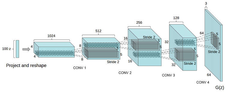
Overview of DCGAN
In recent years, supervised learning with convolutional networks (CNNs) has seen huge adoption in computer vision applications. As compared to supervised learning, ConvNets have received little attention. Deep convolutional generative adversarial networks (DCGANs) have certain architectural constraints and demonstrate a strong potential for unsupervised learning. Training on various image datasets show convincing evidence that a deep convolutional adversarial pair learns a hierarchy of representations from object parts to scenes in both the generator and discriminator. Additionally, the learned features were used for novel tasks — demonstrating their applicability as general image representations.
Problem with GANs
- It’s harder to achieve Nash Equilibrium — Since there are two neural networks (generator and discriminator), they are being trained simultaneously to find a Nash Equilibrium. In the whole process each player updates the cost function independently without considering the updates of cost function by another network. This method cannot assure a convergence, which is the stated objective.
- Vanishing gradient — When the discriminator works as required, the distribution D(x) equals 1 when x belongs to Pr and vice versa. In this process, loss function L fails to zero and results in no gradients to update the loss during the training process. This figure shows that as the discriminator gets increasingly better, the gradient vanishes fast, tending to 0.
- Use better metric of distribution similarity — The loss function as proposed in the vanilla GAN (by Goodfellow et al.) measures the JS divergence between the distributions of Pr and P(theta). This metric fails to provide a meaningful value when two distributions are disjointed.
Replacing JS divergence with the Wasserstein metric gives a much smoother value space.
Training a Generative Adversarial Network faces a major problem:
- If the discriminator works as required, the gradient of the loss function starts tending to zero. As a process loss cannot be updated, training becomes very slow or the model gets stuck.
- If the discriminator behaves badly, the generator does not have accurate feedback and the loss function cannot represent the reality.
Evaluation Metric
GANs faced the problem of good objective function that can give better insight of the whole training process. A good evaluation metric was needed. Wasserstein Distance sought to address this problem.
Few GANs Applications
These are some very few applications of GANs (just to provide some ideas) but they can be extended to do so much than what we can possibly think of. There are many papers which have made use of different architectures of GANs, some are listed below:
- Font generation with conditional GANs
- Interactive image generation
- Image editing
- Human pose estimation
- Synthetic data generation
- Visual saliency prediction
- Adversarial examples (defense vs attack)
- Image blending
- Super resolution
- Image inpainting
- Face aging
Code
The code can be found in this Github* repository.
Empirical Results
Initially the paper (Soumith at al.) demonstrated the real difference between GAN and WGAN. A GAN Discriminator and Wasserstein GAN critic are trained optimality. In the following graph blue depicts real Gaussian distribution and green depicts fake ones then the values are plotted. The red curve depicts the GAN discriminator output.
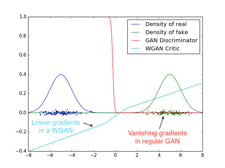
Both GAN and WGAN will identify which distribution is fake and which ones are real, but GAN Discriminator does this in such a way that gradients vanish over this high dimensional space. WGANs make use of weight clamping which gives them an edge and it which is able to give gradients in almost every point in space. Wasserstein loss seems to correlate well with image quality also.
This post was originally written for Intel AI Academy titled as Better Generative modelling through Wasserstein GANs
Visit AI Journal for more videos. Don’t forget to subscribe . Stay connected with us on Twitter to stay updated in AI Research. Please support me on Patreon